To learn from unlabeled data (only inputs, no target information). Most often for classification. Requires that class membership can be detected by structural properties (features) in the data, and that the learning system can be fund these features.
K-means
Following is the algorithm.
 K-means, for K=2
     1. Make a 'codebook' of two vectors, c1 and c2
     2. Sample (at random) two vectors from the data as initial values of c1 and c2
     3. Split the data in two subsets, D1 and D2, where D1 is the set of all points with c1 as their closest codebook vector, and D2 is the corresponding set for c2
     4. Move c1 towards the mean in D1 and c2 towards the mean in D2
     5. Repeat from 3 until convergence (until the codebook vectors stop moving)

This image is copyright by wikimedia.
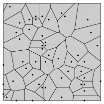
Voronoi regions
-
K-means define Voronoi regions in the input space
-
The Voronoi region around a codebook vector ci is the region in which ci would be the closest codebook vector
This image is copyright by wolfram
Competitive Learning (LVQ-I without neighborhood function)
Goal: Classify N-dimensional data into M classes, i.e. identify M clusters. M nodes, fully connected to the inputs (as usual).
Weight vector = coordinate in the N-dimensional input space ==> Each node has a position.
Changing the weights = moving the node.
Given input vector, x, find the node k which is closest to x (the winner). [the node with the smallest distance between its weight vector and the input vector]. Update node k so that it becomes even more likely to win next time the same input vector shows up, i.e. move it towards the input vector (SHOW):
\Delta \overline{w_{k}}=\eta(\bar{x}-\overline{w_{k}})=\eta\left(x_{i}-w_{k i}\right), 1 \leq i \leq N
$$
This is the standard competitive learning rule
Note: only the winner is moved !
Neural: Find the node with the greatest weighted sum. Same thing if the weight vectors are normalized to unit length. (why the sum is the greatest weighted sum ?)
Competitive learning + batch learning = K-means
The winner-takes-all problem: If a single node wins a lot, it may become invincible.
Solution 1: Initialize the network by drawing vectors from the training set. Solution 2: Modify the distance measure to include the frequency of winning.
Reducing dimensionality
Project data down to lower dimensional space. Have data of high dimensionality. Want to reduce, i.e. project down to some sub space of lower dimensionality, without destroying the class information in the data.
Principal Component Analysis (PCA)
Also known as: Karhunen-Loève transform Idea: Find M orthogonal vectors in the input space, in the directions of greatest variance. Then project the data down to those vectors.
-
First principal component = the direction of largest variance.
-
ith component = direction of largest variance, and orthogonal to the first i–1 components.
Principal components = eigenvectors of the correlation matrix of the input data, corresponding to the M largest eigenvalues.

In a linear MLP with one hidden layer (DRAW), trained as an auto-associator, the M nodes in the hidden layer will approximate the M first principal components. Interesting applications
Kohonens Self Organizing Feature Maps (SOFM)
SOFM: Non-linear, topologically preserving, dimension reduction (compare to a pressed flower, or a photograph).
Idea based on two observations:
-
The cerebral cortex is in effect two dimensional, yet we can reason in more dimensions than two (dimension reduction)
-
Cells in the auditory cortex which respond to certain frequencies, are located in frequency order. (Topological preservation / topographic map)

A 2 (usually) dimensional grid of neurons with common inputs.
Learning: Competitive learning, extended to update not only the winner, k, but also its closest neighbors (structurally, on the grid, not in the input space). [Note: Two different distance concepts – in the weight space and on the grid]
But, we don’t want to update the neighbors as much as the winner. Define a neighborhood function f(j, k) which is 1 for the winner (j = k) and then decreases with the distance (on the grid) from node k.
Examples: Linearly decreasing neighborhood. Gaussian. Mexican hat.
The update rule is a slight modification of the standard competitive learning rule:
\Delta w_{j i}=\eta f(j, k)\left(x_{i}-w_{j i}\right)(\text { for all nodes } j \text { and all inputs } i)
In summary:
-
Find the closest matching node to the input
-
Increase the similarity of this node, and those in the neighborhood, to the input Good idea to decrease neighborhood radius and learning rate over time
After training, the active areas on the map are labelled by presenting patterns for which the generating class is known.

文章评论